packages <- c("readr","tidyverse", "ggplot2", "lme4",
              "GGally", "lmerTest", "MuMIn", "compute.es", "sjPlot", "parameters",
              "HLMdiag","effectsize", "ggpubr", "plotly")

# lattice good for plotting model outputs
# Check which packages are not installed
packages_installed <- packages %in% rownames(installed.packages())

# Install packages not yet installed
for (i in 1:length(packages)) {

  if (packages_installed[i] == FALSE) {
    install.packages(packages[i])
    print(packages[i])
  }
}

## Load packages
lapply(packages, require, character.only = TRUE)

if (sum(packages %in% .packages(TRUE)) < length(packages)) {
  print("Issue loading packages")
} else {
  print("Packages loaded successfully")
}An applied example of a linear mixed model with sport data
Team sport
Data
Statistics
Linear mixed model
Long read (+10 mins)
Using linear mixed models is a powerful way to analyse sports data

The increasing complexity in data collection and its abundance means we must be equipped to answer more complex questions. Linear mixed models provide a flexible and appropriate way to do so. Using R, I will demonstrate how to build a linear mixed model with Australian football training data.
NoteTL;DR
- Why Linear Mixed Models (LMMs): LMMs are well suited to sports data with repeated measures over time, accomodating increasing data complexity and interrelated structures
- How they work: LMMs combine fixed effects (i.e. systematic influences) and random effects (i.e. individual specific variability), allowing increased accuracy and individualised analysis
- Modelling approach: Using R, data are explored and assumptions checked, a null model is built first, then fixed effects are added into the model using a step-up approach, with evaluation using AIC values and statistical significance testing, with model accuracy and applied relevance discussed in a future subsequent part
TipDownloadable file of the article
The file and data I will be using to construct the linear mixed model is also available here:
Estimated reading time: ~15 minutes
Models and Linear Mixed Models
Models in sport science are an extremely useful tool for analysis. Models are primarily built to make inferences and explore phenomenon’s in our data, or to make predictions for future interventions we may make. Often, we want to understand the responses athletes or the team may have in response to manipulations we make in our interventions. For example, we change the field width in a particular drill and want to assess the response in team tactical metrics we collect, or we collect creatine kinase as an indicator of recovery and want to assess the changes in this blood marker over the season after incorporating ice baths one day post-match, or we want to assess how the presence of a swinger/floater influences tactical and technical metrics in some small sided games. The list goes on and on. Here, building models can help us understand how to get the best out of this data for understanding manipulations we make right now but also for future use and ‘expectations’ we may have.
Linear Mixed Models (LMMs) are helpful for allowing practitioners to assess dynamic phenomena over longitudinal timeframes and account for individual characteristics (Krueger & Tian, 2004). LMMs can characterise both individual and group characteristics and differences, simultaneously. Moreover, datasets in sport are typically collected over days, weeks and years, with dependent observations (related datapoints) and are imbalanced (e.g. missing data due to injury, (de)selection, players changing positions between matches etc.) (Newans et al., 2022). Resultantly, mixed modelling provides a robust and flexible method that can assist with these limitations and adjusts the estimates accordingly, providing more accurate and meaningful results.
Furthermore, there is contemporary thinking of behaviour in team sport that is based on complex systems theory. Whilst the evidence to clearly define the links with behaviour and team sport have not fully been established empirically, methods of analysis must now reflect this way of thinking. This may manifest in some of the examples mentioned above but can further be extended to when we don’t have set timeframes/periods between data collections, players that change teams between seasons, different sized grounds as in the AFL or rule changes that affect styles of play and tactics (e.g. 6-6-6 rule; Seakins et al., 2023). Such dynamic changes week-to-week or year-to-year require an adaptive analytical approach, which LMMs provide.
Fixed versus Random Effects
It will become clearer as we start to build our models below, but we should first have an understanding of what fixed and random effects are and how they are different. Importantly, both of these effects are different and are what create the ‘mixed’ element in LMMs. A LMM is a statistical technique that uses both fixed and random effects. The example I will quickly use here to compare fixed and random effects is looking at what factors influence the readiness to perform of soccer players after a match, at 2 different time points (24h and 48h post match). We may have measured variables such as amount and quality of sleep, measures of creatine kinase and a counter movement jump. Here, our counter movement jump is our indicator of recovery and readiness to perform.
Fixed Effects are variables that are treated as being predictable or constant across all levels in the analysis. In other words, they are ‘fixed’ because they have a fixed or systematic influence on the dependent variable. The fixed effects here would include the time (as a factor), the amount of sleep, the quality of sleep and creatine kinase.
Random Effects allow us to solve the inter-dependence problem and not violate the statistical assumption of independent data. Specifying random effects into our LMM allows for a different ‘baseline’ for each level of the random effect. The random effect here would be each player (i.e. each player would have an ID number) and as such, we consider each different players baseline counter movement jump measure. Consequently, specifying player as a random effect captures the variability within each player.
This approach provides a more powerful, flexible and robust method to analyse complex datasets and allows researchers and practitioners to estimate specific variables of interest that can explain a dependent variable (e.g. countermovement jump scores) using fixed effects whilst accounting for the variability within the levels collected (e.g. individual player variation) using random effects.
This article is part one of two. This first part is a guide to prepare your dataset and construct the linear mixed models, whilst the second part will assess the results whilst satisfying assumptions and importantly, understanding the results generated. The analysis here will follow an exploratory project that I haven’t previously analysed. The inspiration for this comes from wanting to provide a sport specific example of building a linear mixed model in a more explanatory, ‘blog’ format.
My understanding of linear mixed models and their constructions can be attributed to performing research in this area (Tribolet et al., 2021; Fransen et al., 2022) and learning about their applications in relation to my own research projects, infinite online searching, and also through Bodo Winters tutorials on building mixed models (Read part one here and and part two here). I’d recommend reading these articles to get a good grasp of linear mixed models and why they are a powerful tool for analysing data.
Data Structure
The main purpose of using linear mixed models is because they are powerful and flexible. The flexibility here provides us with the ability to model repeated measures and maintain a level of power (i.e. maintain information in the dataset rather than remove observations). In sport, we collect multiple measures per athlete. This inherently violates the assumption of independence because the observations and data are INTER-dependent. The following analysis looks at individuals repeated measures across 15 different training conditions in Australian football practice. Hence, the measures are inter-dependent, and a linear mixed model is justified, and necessary.
Here, I want to assess the relationship between a measure of integrative behaviour and traditional metrics and task constraints that we manipulate during practice (e.g. the width of the field, the total number of players in the drill etc). Integrative measures are metrics that show the individuals contribution in the network, or team. The measure I will assess is something called Indegree Importance (Sheehan et al., 2019). This metric is a component score (made up of multiple metrics whilst maintaining the overall variance) and simply reflects the incoming interactions regarding ball movement. Higher values signify that a player is easily reachable, located centrally within the team and is used by more players in the team (Sheehan et al., 2019). You may typically expect forwards and midfielders to have higher scores. The scores are standardised which means the average is 100 and a one standard deviation increase or decrease equals +15 or -15, respectively.
Let’s first upload the key packages we will work with:
readr: upload csv file into R environmentlmer: to build linear mixed modelstidyverse: general suite of packages for data cleaning and wranglingGGally: to assess and visualise any multicollinearityplotly: create interactive plotsggpubr: create and arrange plotslmerTest: testing and comparing models for appropriate fitMuMIn: mixed model assessmentparameters: computing model parameters (confidence intervals, effect sizes)compute.es: computing the effect sizes associated with modelssjPlot: plotting model outcomesHLMdiag: plotting model outcomes
Next, we need to upload the data into R,
# Load data into our workspace
library(readr)
ind_df2 <- read_csv("Individual.xlsx")
and rename our key variables we are looking at. Here, we have:
row_ID: ID of each rowcondition: ID of the conditionplayer: player ID numberspp: space per player in metres squaredwidth: width of the drill in metreslength: length of the drill in metrestotal_players: the total number of players in the drill (both teams)time: the time in the drillindegree: indegree imporancekick_eff: kick efficiency (as a percentage)hb_eff: handball efficiency (as a percentage)goals: the number of goalsmarks: the number of marks
row_id <- ind_df2$Row_ID
condition <- ind_df2$Condition_Identifier
player <- as.factor(ind_df2$Player_ID)
spp <- ind_df2$Space_per_Player
width <- ind_df2$Width
length <- ind_df2$Length
total_players <- ind_df2$Total_Players
time <- ind_df2$Time_Secs
indegree <- ind_df2$Indegree_Quotient_Score
kick_eff <- ind_df2$IND_Kick_Efficiency
goals <- ind_df2$Goals
marks <- ind_df2$Marks

## make NAs 0 in the handball percentage column ----
ind_df2$IND_HB_Efficiency[is.na(ind_df2$IND_HB_Efficiency)] <- 0
hb_eff <- ind_df2$IND_HB_Efficiency

ind_df2$IND_Kick_Efficiency[is.na(ind_df2$IND_Kick_Efficiency)] <- 0
kick_eff <- ind_df2$IND_Kick_Efficiency
Next, I want to show you why we need to use a linear mixed model to analyse this dataset. The following plots show the repeated measurements we have collected on each indvidual player and how there are different numbers of measurements for each player. Additionally, we can see the average value for Indegre Importance for each player and each condition is different. This means that to optimise the accuracy and applicability of this data to explain our Indegree Importance numbers, we should use a statistical approach that can help explain the baseline differences at both player and condition levels (and specify them as random effects when we build our models).
## Plots
# repeated measures by player
library(tidyverse) # needed to build plots using ggplot
ggplot(ind_df2, aes(player, indegree)) +
  geom_point(size = 3,
             shape = 21,
             fill = "grey",
             color = "black") +
  theme_classic() +
  theme(axis.text.x = element_text(angle = 60, hjust = 1, vjust = 1)) +
  ylab("Indegree Importance") + xlab("Player") +
  labs(title = "Repeated measures by player",
       subtitle = "Indegree by Player",
       caption = "Figure 1. We see that there are players with only 1 observation (player 19),
       whilst some have 2 observations (players 3 and 25) and others have more (e.g. player 12 has 12 obs)")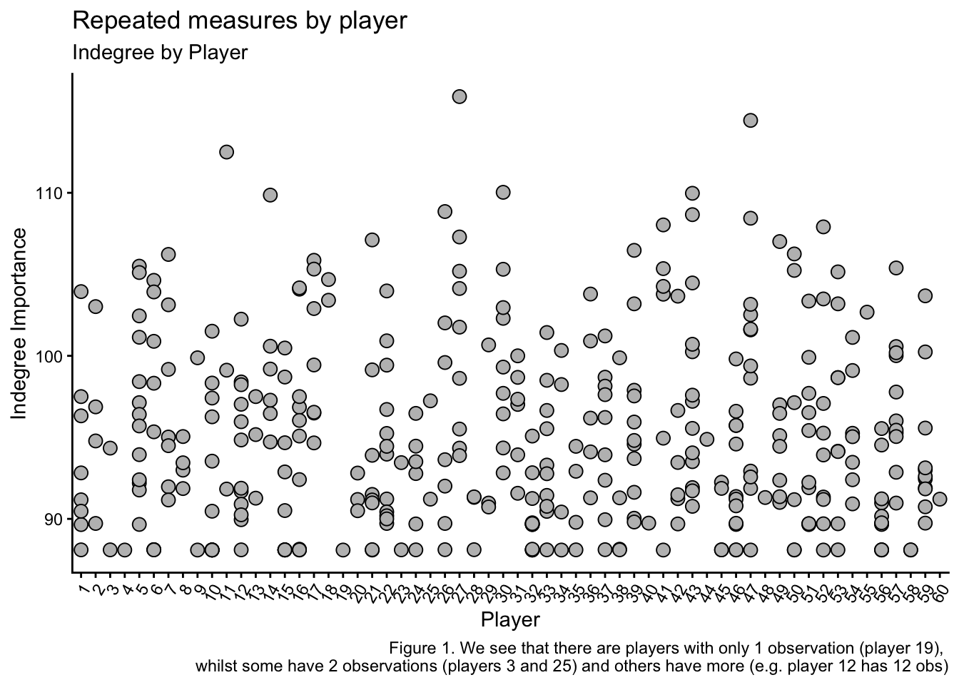
# variation by individual
ggplot(ind_df2, aes(player, indegree)) +
  geom_boxplot() +
  theme_classic() +
  ylab("Indegree Importance") + xlab("Player") +
  theme(axis.text.x = element_text(angle = 60, hjust = 1, vjust = 1)) +
  labs(title = "Box plot variation by player",
       subtitle = "Shows the variation for Indegree Importance for each player",
       caption = "Figure 2. We see different amounts of variation for each player.
       Note that players with 1 observation look like a bold horizontal line")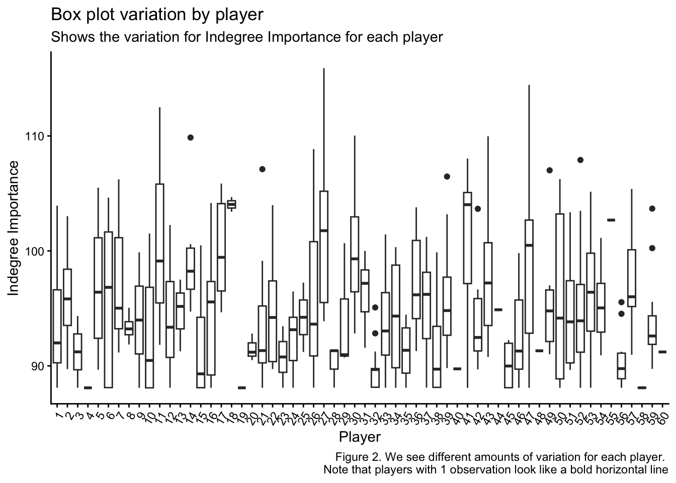
# variation by condition
ggplot(ind_df2, aes(group = condition, indegree)) +
  geom_boxplot() +
  ylab("Condition") + xlab("Indegree Importance") +
  scale_y_continuous(breaks = c(1:15)) + theme_classic() +
  labs(title = "Box plot variation by condition",
       subtitle = "Show the variation for Indegree Importance for each condition",
       caption = "Figure 3. We see different amounts of variation for each condition
       Note that even though we standardised scores for Indegree, there is variation
       in the average across the conditions")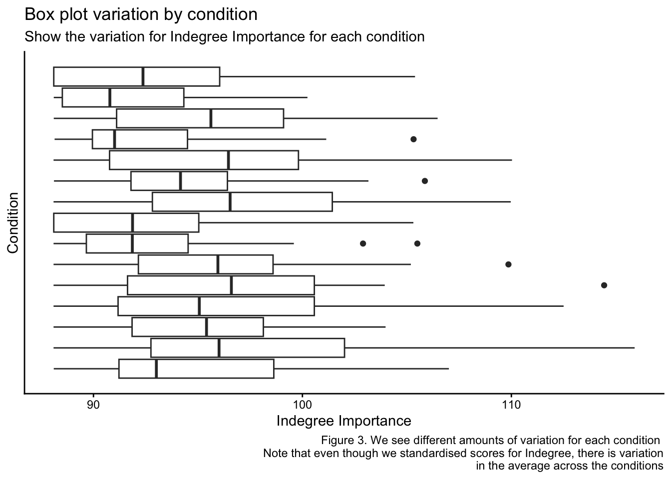
After observing these plots, it should be a little clearer to see why we need to construct our model to account for individual and conditional level relationships. As there is a baseline variation due to each player and each conditions idiosyncrasies, we must account for these to improve our model outcomes and estimations. I will speak about this more during the model construction.
Assumptions
All statistical assessments assume some characteristics about the data you are analysing. These are broadly called assumptions. We must acknowledge and evaluate these assumptions in our data, otherwise we may affect our ability to confidently make conclusions about what the data is saying (in the way of inaccuracy, biased or inflated outcomes), as the results are essentially unreliable and misleading. Next, we will go through and evaluate each of the assumptions relevant to a linear mixed model.
There are a few assumptions for LMMs that we must check to see if our model fits the data well: 1. Independence 2. Linearity of predictors 3. Multicollinearity 4. Normality of residuals (performed after model construction) 5. Homoskedasticity (performed after model construction) 6. Influential datapoints (although not an assumption, it should be an important check performed on the results)
Independence
We have already established that our data is repeated and dependent (Figures 1, 2 & 3). Each data point for each player is related. Hence, our data already violates this assumption. Consequently, we must use a linear mixed model, which can be used when independence is violated.
Linearity
Next in our data structure is the relationships between our predictor variables with Indegree Importance. This relates to the assumption of linearity. After all, they are called linear mixed models, so the relationship between our predictors and Indegree Importance generally needs to be linear. Our predictor variables are investigating the impact or influence on Indegree Importance. They include drill width, drill length, space per player, the total number of players, time, handball efficiency, kick efficiency, marks and goals.
library(ggpubr)
# indegree by width
p1 <- ggplot(ind_df2, aes(width, indegree)) +
  geom_point() +
  geom_smooth(method = "lm") +
  stat_cor(method = "pearson") + ## show correlation value
  ylab("Indegree") + xlab("Width (m)") +
  theme_classic() +
  labs(title = "Width (m) and
Indegree Importance")

# indegree by length
p2 <- ggplot(ind_df2, aes(length, indegree)) +
  geom_point() +
  geom_smooth(method = "lm") +
  stat_cor(method = "pearson") + ## show correlation value
  ylab("Indegree") + xlab("Length (m)") +
  theme_classic() +
  labs(title = "Length (m) and
Indegree Importance")

# indegree by space per player
p3 <- ggplot(ind_df2, aes(spp, indegree)) +
  geom_point() +
  geom_smooth(method = "lm") +
  stat_cor(method = "pearson") + ## show correlation value
  ylab("Indegree") + xlab("Space per Player (m2)") +
  theme_classic() +
  labs(title = "Space per player (m2)
and Indegree Importance")

# indegree by total number of players
p4 <- ggplot(ind_df2, aes(total_players, indegree)) +
  geom_point() +
  geom_smooth(method = "lm") +
  stat_cor(method = "pearson") + ## show correlation value
  ylab("Indegree") + xlab("Total Players (n)") +
  theme_classic() +
  labs(title = "Total number of players (n)
and Indegree Importance")


## arrange all of the above plots into 1 image for simplicity
ggarrange(p1, p2, p3, p4, ncol = 2, nrow = 2, labels = c("A", "B", "C", "D"))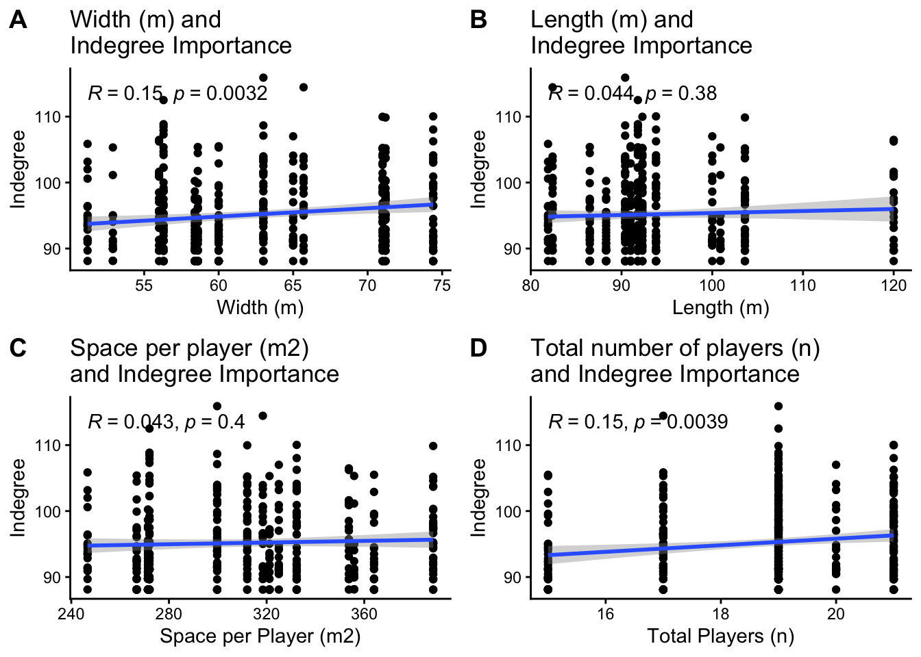
## Although I won't perform it here, check the general linearity of time,
## handball and kick efficiency, marks and goals.
## The process is the same as above
Multicollinearity
Next, we must also consider multicollinearity in our dataset. Multicollinearity is when two variables are highly correlated. If we don’t investigate multicollinearity, we can’t separate and interpret the effects of each one of the variables. Additionally, we must assess this to make sure we aren’t inflating what is called a type I error – finding significant and meaningful effects in the data when they don’t actually exist. For example, say we want to measure the things that contribute to the number of disposals a player accumulates in a game. We measure kicks, handballs, goals and behinds (goals and behinds are kicks of course). Here, it is likely that the relationship between kicks and handballs with disposals is quite high, because they both contribute to the same measure. As such, a correlation sees them as ‘the same thing’ statistically. If the relationship/correlation between the two measures is over 0.8, they are statistically ‘the same variable’, and as such, we need to remove one. Otherwise, we inflate the chance of finding something significant by essentially building the model with the same metric twice.
Consequently, we are looking for collinearity between our predictor values (as previously listed). We will use the GGally package to visualise the correlations in our dataset in a correlation matrix.
p5 <- GGally::ggcorr(ind_df2[,6:29], size = 2, label = TRUE, label_round = 2, label_size = 2)
plotly::ggplotly(p5)
# no collinearity between our predictors, so we can include each of them together if requiredUsing our predictor variables, there are no concerns of multicollinearity that we can see here. However, if we were using both Handball totals (HB_Total) and handball efficiency (HB_Eff) as predictors in our model, we would have to remove one of them due to the high correlation (dark red colour, value = 0.94). Hence we would have to remove one from our analysis. Here, we would assess which one is more highly correlated with Indegree Importance and keep the one that has the higher correlation value.
Now that we have established there are no violations of any assumption, we can continue with our model constructions.
Model Construction
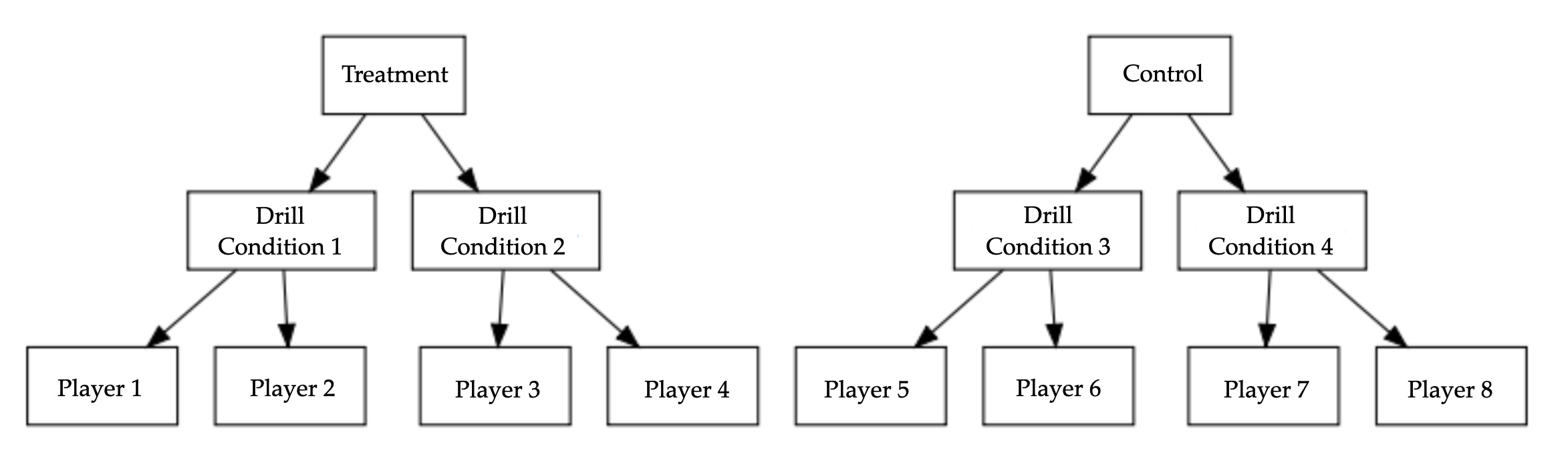
Firstly, we build what’s called a null model (it is a null model with a random intercept). In data structures with hierarchical data (Figure 4), there are levels to the data. Here, we have players within condition. There is a grouping variable (i.e. the practice drill) and each player within the drill. Here, the null model serves to confirm if multi-level modelling is necessary. In this case, we are assessing if having player AND condition specified and built as random effects is necessary. It also serves as a ‘baseline’ model with no predictors so we can assess the random effects only.
We use the lmer function, followed by our dependent variable (Indegree Importance) as a function of 1 that also factors individual differences in players into the formula. In other words, our formula is specifying Indegree Importance predicted by 1, that accounts for different ‘baselines’ according to player. We also want to see if the condition (i.e. each practice drill) can provide some use and explanatory power to our model, so we build the below models. Logically, the second model should provide more utility than the first, assuming that each player AND each condition will have varying baselines compared to not having varying baselines. Visually, we know this is the case as we saw it in the boxplots graph above (Figure 3). If there is a lower AIC value and statistical significance, the models are statistically different, and we retain the model with the lower AIC values and statistical significance. We will use the anova() function to compare the two models.
library(lmerTest)
## Our two null models are as follows:
null_model1 <- lmer(indegree ~ 1 + (1|player)) ## only player specified as a random effect
null_model2 <- lmer(indegree ~ 1 + (1|player) + (1|condition)) ## both player and condition specified as random effects

anova(null_model1, null_model2)
Data: NULL
Models:
null_model1: indegree ~ 1 + (1 | player)
null_model2: indegree ~ 1 + (1 | player) + (1 | condition)
npar AIC BIC logLik -2*log(L) Chisq Df Pr(>Chisq)
null_model1 3 2418.8 2430.6 -1206.4 2412.8
null_model2 4 2406.6 2422.4 -1199.3 2398.6 14.17 1 0.000167 ***
---
Signif. codes: 0 '***' 0.001 '**' 0.01 '*' 0.05 '.' 0.1 ' ' 1(Note that I also tried a null model that looked at whether it would be a better fit if player observations were nested within each condition. This is a more complex random effects structure, so I won’t explain it here. But it didn’t provide a better model fit, so I discarded it)
This output initially shows our models that we are comparing. You obtain an AIC value and a p-value from the comparison of the two models, which is showing that the inclusion of condition as a random effect makes the model statistically different to the model with just player as a random effect. Consequently, because the condition is the only variable that differs between the two models, we can conclusively say that condition statistically influences Indegree Importance. As such, we retain this baseline model:
Before we start to construct our models using the predictor variables, I want to check the normality of our residuals in this baseline model. This is one of our assumptions and a violation indicates a poorly fit model which means lowered accuracy and lower applicability of the model.
plot(fitted(null_model2), resid(null_model2), abline(h = 0), ylim = c(-20, 20))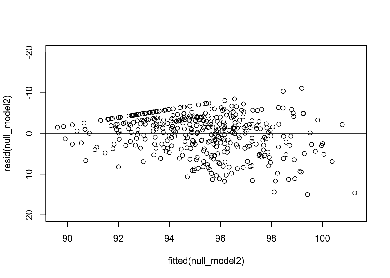
The plot shows a general pattern. That being, small errors at smaller fitted values and larger errors at large fitted values. This may reflect a violation of linearity in our null model. There is also a ‘straight line’ of error values across the top of the datapoints. Which is quite strange but we will see how this changes as we build then assess our models. Let’s continue to see how both these things change as we fit further variables into our model in the way of fixed effects.
As this model and analysis is exploratory, we will use a step-up model construction approach. This approach has been popular in sports research (Kempton & Coutts, 2016; Dillon et al., 2017; Henderson et al., 2019; Tribolet et al., 2021). Firstly, the baseline model (we will start with our null model) is compared to the next model with the singular addition of 1 fixed effect. This way, we can conclusively state that the included fixed effect is statistically the difference or not. If we include two or more fixed effects, we don’t know which one is statistically contributing to the model. We will use the lme4 (Bates et al. 2015) and lmerTest (Kuznetsova et al. 2017) packages to construct and assess our models.
Let’s start with our variables that correlate highly with indegree scores (marks, handball efficiency, kick efficiency and shots on goal). For model 1, we will add marks as a fixed effect.
model1 <- lmer(indegree ~ marks + (1|player) + (1|condition), REML=FALSE)
null_model2 <- lmer(indegree ~ 1 + (1|player) + (1|condition))
anova(model1, null_model2)
refitting model(s) with ML (instead of REML)Data: NULL
Models:
null_model2: indegree ~ 1 + (1 | player) + (1 | condition)
model1: indegree ~ marks + (1 | player) + (1 | condition)
npar AIC BIC logLik -2*log(L) Chisq Df Pr(>Chisq)
null_model2 4 2406.6 2422.4 -1199.3 2398.6
model1 5 2299.8 2319.6 -1144.9 2289.8 108.79 1 < 2.2e-16 ***
---
Signif. codes: 0 '***' 0.001 '**' 0.01 '*' 0.05 '.' 0.1 ' ' 1The comparison using an ANOVA shows lower AIC and a statistically significant difference for model 1. Consequently, we continue with model 1 and continue to add more fixed effects with this model as our baseline. To be clear, model 1 may colloquially read as “Indegree predicted by marks, that caters for each players and conditions baseline”.
In addition to marks, we will now also add handball efficiency into the next model.
model2 <- lmer(indegree ~ marks + hb_eff + (1|player) + (1|condition), REML=FALSE)
anova(model1, model2)
Data: NULL
Models:
model1: indegree ~ marks + (1 | player) + (1 | condition)
model2: indegree ~ marks + hb_eff + (1 | player) + (1 | condition)
npar AIC BIC logLik -2*log(L) Chisq Df Pr(>Chisq)
model1 5 2299.8 2319.6 -1144.9 2289.8
model2 6 2271.9 2295.7 -1130.0 2259.9 29.853 1 4.661e-08 ***
---
Signif. codes: 0 '***' 0.001 '**' 0.01 '*' 0.05 '.' 0.1 ' ' 1The comparison using an ANOVA shows lower AIC and significant difference for model 2. We continue with model 2. To be clear, model 2 may colloquially read as “Indegree predicted by marks and handball efficiency, that caters for each players and conditions baseline”.
We will now add kick efficiency.
model3 <- lmer(indegree ~ marks + hb_eff + kick_eff + (1|player) + (1|condition), REML=FALSE)
anova(model2, model3)
Data: NULL
Models:
model2: indegree ~ marks + hb_eff + (1 | player) + (1 | condition)
model3: indegree ~ marks + hb_eff + kick_eff + (1 | player) + (1 | condition)
npar AIC BIC logLik -2*log(L) Chisq Df Pr(>Chisq)
model2 6 2271.9 2295.7 -1130 2259.9
model3 7 2268.1 2295.8 -1127 2254.1 5.8543 1 0.01554 *
---
Signif. codes: 0 '***' 0.001 '**' 0.01 '*' 0.05 '.' 0.1 ' ' 1The comparison using an ANOVA shows slightly lower AIC and significant differences for model 3. We continue with model 3.
model4 <- lmer(indegree ~ marks + hb_eff + kick_eff + goals + (1|player) + (1|condition), REML=FALSE)
anova(model3, model4)
Data: NULL
Models:
model3: indegree ~ marks + hb_eff + kick_eff + (1 | player) + (1 | condition)
model4: indegree ~ marks + hb_eff + kick_eff + goals + (1 | player) + (1 | condition)
npar AIC BIC logLik -2*log(L) Chisq Df Pr(>Chisq)
model3 7 2268.1 2295.8 -1127.0 2254.1
model4 8 2269.3 2300.9 -1126.7 2253.3 0.7774 1 0.3779Here is our first instance where we reject the new model construction (i.e. model 4). This is based on a higher AIC value and not being statistically different to model 3. This is saying that adding how many goals each player has does not statistically improve the prediction of Indegree Importance. As such, we can discard this model. We then continue again with model 3.
model5 <- lmer(indegree ~ marks + hb_eff + kick_eff + width + (1|player) + (1|condition), REML=FALSE)
anova(model3, model5)
Data: NULL
Models:
model3: indegree ~ marks + hb_eff + kick_eff + (1 | player) + (1 | condition)
model5: indegree ~ marks + hb_eff + kick_eff + width + (1 | player) + (1 | condition)
npar AIC BIC logLik -2*log(L) Chisq Df Pr(>Chisq)
model3 7 2268.1 2295.8 -1127.0 2254.1
model5 8 2269.3 2300.9 -1126.7 2253.3 0.7815 1 0.3767Similar to the model 4, model 5 has a higher AIC and is not statistically different to model 3. Similar to model 4, the width of the drill does not predict or influence a players level of Indegree Importance. As such, we can discard this model.
model6 <- lmer(indegree ~ marks + hb_eff + kick_eff + total_players + (1|player) + (1|condition), REML=FALSE)
anova(model3, model6)
Data: NULL
Models:
model3: indegree ~ marks + hb_eff + kick_eff + (1 | player) + (1 | condition)
model6: indegree ~ marks + hb_eff + kick_eff + total_players + (1 | player) + (1 | condition)
npar AIC BIC logLik -2*log(L) Chisq Df Pr(>Chisq)
model3 7 2268.1 2295.8 -1127.0 2254.1
model6 8 2267.6 2299.2 -1125.8 2251.6 2.4813 1 0.1152Model 6 shows slighlty lower AIC, but no statistically significant difference between the two models. There is an argument to continue with model 3 here, as the addition of total players hasn’t provided statistically different findings when we compare the two models. Additionally, they are essentially the same model statistically, but model 6 is more complex as it has one more variable than model 3. As such, we need to make a choice between which model to continue with. There is some practicality keeping the total players variable in the model as it provides a ‘tangible’ manipulation we can make during practice.
I want to continue with model 6, which includes the total players.
model7 <- lmer(indegree ~ marks + hb_eff + kick_eff + total_players + time + (1|player) + (1|condition), REML=FALSE)
anova(model6, model7)
Data: NULL
Models:
model6: indegree ~ marks + hb_eff + kick_eff + total_players + (1 | player) + (1 | condition)
model7: indegree ~ marks + hb_eff + kick_eff + total_players + time + (1 | player) + (1 | condition)
npar AIC BIC logLik -2*log(L) Chisq Df Pr(>Chisq)
model6 8 2267.6 2299.2 -1125.8 2251.6
model7 9 2269.5 2305.1 -1125.7 2251.5 0.1233 1 0.7255Model 7 has a higher AIC and isn’t statistically different, so we can discard it and keep model 6.
Model Applicability and Comparison
After we are happy with our model and the process of constructing it, we must assess a few things. Before that, let’s recap what information we have with our model so far.
Here, Indegree Importance is being predicted by marks, handball efficiency, kick efficiency and total players in the drill. These variables are what we call fixed effects, which have systematic or a fixed effect on Indegree Importance. We have also included player AND condition as random effects. Here, these random effects characterise the idiosyncrasies due to player and condition differences (as we saw above when we looked at the boxplots of each player and condition; Figures 1, 2 and 3). This mixture of fixed and random effects is what makes the mixed model a mixed model. We have reached this model by comparing a full model (with the fixed effects in question) against a reduced model without the fixed effects question. We have used the anova() function to compare models and subsequently continued with the model if it had a lower AIC value and was statistically different. However, model6 (our current model just above) only had a slightly lower AIC compared to model3 using the step-up approach. I kept it as it has a slightly lower AIC and the practicality of having the fixed effects included seemed useful. This is where understanding the data and having knowledge from the field and area you work in is crucial. Is it worth retaining a variable when it may make the model more complex? The knowledge of the practitioner/researcher is crucial.
Before we assess the results of our final model and summarise our findings, we must first check some assumptions of the ‘fit’ of our model (i.e. how suitable are the predictions, or the fitted values of the model) and ensure it does not violate some key assumptions. This will be in the second part of this article, which will be published separately.
Conclusion
Linear mixed models are a powerful and flexible way to analyse sports data. The inclusion of both fixed and random effects allow practitioners and researchers the possibility to appropriately analyse datasets with repeated measures, missing data and longitudinal data to help increase the accuracy and practicality of the findings. We must firstly meet the relevant statistical assumptions to ensure our findings are unbiased, reliable and accurate. We can then build a null (i.e. base) model and then use a step-up construction method to add fixed effects (predictor variables) to assess their affect on our dependent variable (i.e. Indegree Importance).
References
Bates D, Maechler M, Bolker B, Walker S. 2015. Fitting linear mixed-effects models using lme4. J Stat Softw. 67(1):1–48. doi:10.18637/jss.v067.i01.
Crueger, C. & Tian, L. (2004), A comparison of the general linear mixed model and repeated measures ANOVA using a dataset with multiple missing data points, Biological Research for Nursing, 10.1177/1099800404267682.
Dillon P.A., Kempton, T., Ryan, S., Hocking, J. & Coutts, A.J. (2017), Interchange rotation factors and player characteristics influence physical and technical performance in professional Australian Rules football, Journal of Science and Medicine in Sport, 21(3), 317-321.
Fransen, J., Tribolet, R., Sheehan, W.B., McBride, I., Novak, A.R. & Watsford, M.L. (2022), Cooperative passing network features are associated with successful match outcomes in the Australian Football League, International Journal of Sports Science and Coaching, 10.1177/17479541211052760.
Henderson, M.J., Fransen, J., McGrath, J.J., Harries, S.K., Poulos, N. & Coutts, A.J. (2019), Situational factors affecting rugby sevens match performance, Science and Medicine in Football, 10.1080/24733938.2019.1609070.
Kempton, T. & Coutts, A.J. (2016), Factors affecting exercise intensity in professional rugby league match-play, Journal of Science and Medicine in Sport, 19(6), 504-508.
Kuznetsova A, Brockhoff PB, Christensen RHB. 2017. lmerTest package: tests in linear mixed effects models. J Stat Softw. 82(13):1–26. doi:10.18637/jss.v082.i13.
Newans, T., Bellinger, P.M. & Drovandi, C.C. (2022), The utility of mixed models in sports science: A call for further adoption in longitudinal datasets, International Journal of Sports Physiology and Performance, doi.org/10.1123/ijspp.2021-0496.
Seakins, D., Gastin, P., Jackson, K., Gloster, M., Brougham, A. & Carey, D.L. (2023), Discovery and Characterisation of Forward Line Formations at Centre Bounces in the Australian Football League, Sensors, 10.3390/s23104891.
Sheehan, W.B., Tribolet, R., Watsford, M.L., Novak, A.R., Rennie, M.J. & Fransen, J. (2019), Using cooperative networks to analyse behaviour in professional Australian Football, Journal of Science and Medicine in Sport, doi.org/10.1016/j.jsams.2019.09.012.
Tribolet, R., Sheehan, W.B., Watsford, M.L., Novak, A.R. & Fransen, J. (2021), Factors associated with cooperative network connectedness in a professional Australian football small-sided game, Science and Medicine in Football, doi.org/10.1080/24733938.2021.1991584.
▲ Back to top